![]()
Inhoud:
1. Doel en strekking / Purpose and scope
4. Benodigdheden / requirements
5.1.
Algemene aanwijzingen / general instructions
5.2.7.
Handmatig invoeren / Manual entry
PLA tredecim als Excel-applicatie: 27-Dec-2018 01:09:18
1.
Doel en
strekking / Purpose and scope
|
Dit document is de handleiding en bevat de Microsoft Excel worksheet
“PLA in Excel”. |
This document is the manual and contains the
Microsoft Excel worksheet “PLA in Excel”. |
2.
Inleiding /
Introduction
|
Deze PLA (parallel line assay) rekenmethode is in Microsoft
Excel-worksheet geprogrammeerd. Deze applicatie leest ELISA-plaatbestanden in en vult, tot dertien
monsters, per monster een PLA-tabblad met gegevens. De resultaten van deze
dertien tabbladen worden gegroepeerd in een tabel en voorzien van een kleur,
afhankelijk of de statistiek binnen of buiten specificaties valt. Deze PLA-rekenmethode is beschreven door Finney en wordt toegepast in
dilution assays. Bij deze bepalingen wordt de respons gemeten per verdunning
van een test monster en vergeleken met de respons van dezelfde verdunningen
van standaard. Door middel van een variantieanalyse wordt aan de hand van
F-toetsen en betrouwbaarheid van de berekende potency de validiteit van het
resultaat getoetst. |
This PLA (parallel line assay) calculation method is
programmed in Microsoft Excel. The program is designed to calculate up to thirteen
potencies from data measured in a 8 by 12 ELISA format or from linear lists
with data. Results are grouped per sample on thirteen separated sheets or
grouped together in one sheet. Depending on the calculated statistics results
are flagged with a colour to identify results with statistical results out of
specification. The PLA calculation method followed was written by
Finney and is designed dilutions assays. The measured response of a dilution
of a test sample is compared with the response of the same dilution of a
standard. By means of analysis of variance a F-test is calculated and used to
validate the calculated potency of the test sample. |
3.
Principe /
Principle
|
Het uitgangspunt van de PLA-berekening is dat de logaritme
van de dosis een lineair verband vertoont met de gemeten respons. De parallel line assay is een variant van de slope ratio assay (SRA)
waar doses uitgezet op een lineaire schaal en responsen een lineair
verband vertonen. In tegenstelling tot de SRA is bij de PLA geen
gemeenschappelijk snijpunt van de blancometing. Bij testen berekend met de PLA-rekenmethode dient de respons zich dus
lineair te verhouden met de logaritme van de toegevoegde dosis. Het meetgebied
dient zo gekozen te zijn dat standaard en monster hierin een lineair verband
vertonen. Essentieel is ook dat de hellingen van de twee berekende lijnen
overeenkomen. |
The PLA calculation is based on the fact that
the logarithm of the dose has a linear relationship with the
measured response. The parallel line assay is a variant of the slope
ratio assay (SRA) where doses are plotted on a linear scale and
responses have a linear relationship with the doses. In contrast with SRA, the PLA does not have a common
intersection of the blank measurement. In tests using the PLA calculation method, the
response must therefore be linear in relation to the logarithm of the added
dose. The measuring range must be chosen such that standard and sample herein
have a linear relationship. It is also essential that the slopes of the two
calculated lines are match. |
|
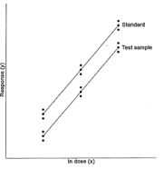
De parallel line assay is in zoverre vergelijkbaar met de slope ratio
assay dat het beide indirecte analytische rekenmethoden zijn. Zij berekenen
een verhouding tussen de standaard en het onbekende testmonster. Met de PLA-rekenmethode wordt de afstand van twee regressie-lijnen,
één regressielijn door de dose-responspunten van de standaard en één
regressielijn door de meetpunten van het testmonster, vergeleken. |
|
Both SRA and PLA are indirect analytical calculation
methods. They calculate a ratio between the potencies of standard and sample. With PLA a distance between two regression lines is
calculated, one thought the standard dose-response points and one regression
line through the dose-response points of the sample |
|
De verhouding van de afstand van de twee parallelle lijnen is de
relatieve potency van het testmonster ten opzichte van de gebruikte standaard.
De respons is een waarde hoeveel keer geconcentreerder of actiever het
testmonster is ten opzichte van de standaard. |
The ratio of the distance of the two parallel lines
is the relative potency of the sample tested in relation to the used standard. Response is an amount of how much concentrated or
more active the sample is in relation to the standard. |
|
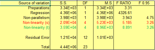
Door middel van variantieanalyse (ANOVA) van de gemeten, meervoudige,
responses per dosis (duplo, triplo, enz.) wordt getest op lineariteit en
parallelliteit van de twee regressielijnen; lopen ze parallel en zijn ze
recht. Variantieanalyse kan niet worden toegepast op enkelvoudige metingen van
een dosis. Samen met de relatieve slope (helling) tussen beide berekende hellingen van de
test wordt de validiteit van de test beoordeeld. Bij de relatieve slope wordt er van uitgegaan dat de twee berekende
hellingen, gedeeld op elkaar, 1.0 is, dus een gelijke helling. Een spreiding van +/-10% wordt algemeen geaccepteerd, de relatieve
helling moet dan tussen de 0.9 en 1.1 liggen. Afhankelijk van de testmethode
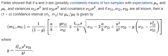
kunnen deze acceptatiegrenzen aangepast worden. Het 95%
betrouwbaarheidsinterval van het resultaat wordt berekend met de stelling van
Fieller. |
By means of analysis of variance (ANOVA) of the
measured responses of replicates of the standard and sample dilutions the
linearity and parallelism is tested. Are the lines straight and are they
calculated parallel to each other. ANOVA cannot be performed on single measurements of
dilutions. A test is validated on the results of the
F-statistics and the calculated relative slope. The relative slope is the
slope of the standard divided by the slope of the sample. This is almost
identical to the test on parallelism but now it is a value that can be judged.
A deviation of 10% is acceptable. Therefore the relative slope must be between
0.9 and 1.1. The 95% confidence interval of the result is
calculated using Fieller's theorem. |
|
Het gebruik van de PLA-rekenmethode heeft als voordeel dat
over meerdere verdunningen van een testmonster één resultaat berekend wordt en
door middel van variantieanalyse een uitspraak wordt gedaan over de kwaliteit
van het resultaat. Het berekende resultaat wordt afgekeurd als een toets
buiten de statistische grenzen valt. Het nadeel van PLA vergeleken met de
logit-regressiemethode is dat het meetbereik vaak erg klein is. Alleen het
lineaire gedeelte van de test kan worden gebruikt. Om deze tekortkoming te
minimaliseren kan in dit programma een algoritme voor logit-optimalisatie
worden gebruikt. Dit zal een sigmoïde curve lineair maken. Een simpele PLA-berekening in Excel is in Tabel 1
weergegeven. Een uitgebreide beschrijving van de rekenmethode is
beschreven in Statistical Methods in Biological Assay" van D.J.
Finney |
The use of the PLA calculation method has the
advantage that one result is calculated over several dilutions of a test
sample and a statement about the quality of the result is made by means of
analysis of variance. The calculated result is rejected if a test falls
outside the statistical limits. The disadvantage of PLA compared to the logit
regression method is that the measuring range is often very small. Only the
linearized part of the test can be used. To minimize this shortcoming a logit
optimise algorithm can be used in this program. This will linearize a sigmoid
curve. A simple PLA calculation in Excel is shown in Table
1. A detailed description of the calculation method is
described in Statistical Methods in Biological Assay "by D.J. Finney |
Tabel 1 PLA without
ANOVA
|
|
A |
B |
C |
D |
E |
F |
|
1 |
x |
y |
log(x) |
x^2 |
x*y |
|
|
2 |
||||||
|
3 |
4 |
1 |
=LOG(A3) |
=C3*C3 |
=C3*B3 |
|
|
4 |
8 |
2 |
=LOG(A4) |
=C4*C4 |
=C4*B4 |
|
|
5 |
16 |
3 |
=LOG(A5) |
=C5*C5 |
=C5*B5 |
|
|
6 |
32 |
4 |
=LOG(A6) |
=C6*C6 |
=C6*B6 |
|
|
7 |
|
|
|
|
||
|
8 |
=SUM(B3:B6) |
=SUM(C3:C6) |
=SUM(D3:D6) |
=SUM(E3:E6) |
||
|
9 |
=COUNT(A3:A6)
nS
|
=B8/$A$9
SyS |
=C8/$A$9
SxS |
=D8-C8^2/$A$9
SxxS |
=E8-B8*C8/$A$9 SxyS |
=E9/D9 RS |
|
10 |
||||||
|
11 |
1 |
1 |
=LOG(A11) |
=C11*C11 |
=C11*B11 |
|
|
12 |
2 |
2 |
=LOG(A12) |
=C12*C12 |
=C12*B12 |
|
|
13 |
4 |
3 |
=LOG(A13) |
=C13*C13 |
=C13*B13 |
|
|
14 |
|
|
|
|
||
|
15 |
=SUM(B11:B13) |
=SUM(C11:C13) |
=SUM(D11:D13) |
=SUM(E11:E13) |
||
|
16 |
=COUNT(A11:A13)
nT |
=B15/$A$16
SyY |
=C15/$A$16
SxT |
=D15-C15^2/$A$16 SxxT |
=E15-B15*C15/$A$16 SxyT |
=E16/D16
RT |
|
17 |
||||||
|
18 |
Slope: |
=(E9+E16)/(D9+D16) |
relative.slope: |
=F16/F9 |
Potency: |
=D19/D20 |
|
19 |
y0 |
=B9-$B$18*C9 |
x0 |
=10^(-B19/$B$18) |
||
|
20 |
y1 |
=B16-$B$18*C16 |
x1 |
=10^(-B20/$B$18) |
En de resultaten.
|
1 |
x |
y |
log(x) |
x^2 |
x*y |
|||
|
2 |
||||||||
|
3 |
4 |
1 |
0.6021 |
0.3625 |
0.6021 |
|||
|
4 |
8 |
2 |
0.9031 |
0.8156 |
1.8062 |
|||
|
5 |
16 |
3 |
1.2041 |
1.4499 |
3.6124 |
|||
|
6 |
32 |
4 |
1.5051 |
2.2655 |
6.0206 |
|||
|
7 |
|
|
|
|
||||
|
8 |
10.0000 |
4.2144 |
4.8934 |
12.0412 |
||||
|
9 |
4 |
2.5000 |
1.0536 |
0.4531 |
1.5051 |
3.3219 |
||
|
10 |
||||||||
|
11 |
1 |
1 |
0.0000 |
0.0000 |
0.0000 |
|||
|
12 |
2 |
2 |
0.3010 |
0.0906 |
0.6021 |
|||
|
13 |
4 |
3 |
0.6021 |
0.3625 |
1.8062 |
|||
|
14 |
= |
= |
= |
= |
||||
|
15 |
6.0000 |
0.9031 |
0.4531 |
2.4082 |
||||
|
16 |
3 |
2.0000 |
0.3010 |
0.1812 |
0.6021 |
3.3219 |
||
|
17 |
||||||||
|
18 |
slope: |
3.3219 |
rel.slope: |
1.0000 |
potency: |
4.0000 |
||
|
19 |
y0 |
-1.0000 |
x0 |
2.0000 |
||||
|
20 |
y1 |
1.0000 |
x1 |
0.5000 |
||||
|
18 |
slope: |
3.3219 |
Relative slope: |
1.0000 |
potency: |
4.0000 |
||
|
19 |
y0 |
-1.0000 |
x0 |
2.0000 |
||||
|
20 |
y1 |
1.0000 |
x1 |
0.5000 |
||||
|
SxS = Σ Log(xS) / nS SyS = Σ Log(xS) / nS SxxS = Σ(Log(xS) * Log(xS)) / nS SxyS = Σ(Log(xS) * yS)
/ nS RS
= SxyS/SxxS SxT = Σ Log(xT) / nT SyT = Σ Log(xT) / nT SxxT = Σ(Log(xT) * Log(xT)) / nT SxyT = Σ(Log(xT) * yT)
/ nT RT
= SxyT/SxxT |
Slope
= (SxyS+SxyT) / (SxxS+SxxT) Relative slope = RS/RT y0
= SyS / (Slope * SxS y1
= SyT / (Slope * SxT x0
= 10^ ( y0 / Slope) x1
= 10^ (-y1 / Slope) Potency
= x0 / x1 |
4.
Benodigdheden /
requirements
·
PLA tredecim V01Aug2018.xlsm.
·
Windows 7 of Windows 10
·
Microsoft
Excel 2010 – 2019
5.
Uitvoering /
performance
5.1. Algemene aanwijzingen /
general instructions
|
De macro’s moeten actief zijn om de worksheet te
kunnen gebruiken. Als dit niet het geval is waarschuwt de worksheet bij
opstarten met een beveiligingswaarschuwing. Ga dan in Files -. Options -> Trust center -> Trust center settings ->
Macro settings en zet “Enable all macros” aan. Start geen documenten van onbekende bronnen of zet de
optie Disable all macros with
notifications” weer aan |
Macros should be enabled for the calculations to run. If this is not the case, the worksheet warns you when
starting with a security warning. Then go in Files -. Options -> Trust center -> Trust
center settings -> Macro settings and enable “Enable all macros”. Be aware that security is low. Do not open documents of unknow source or turn on
“Disable all macros with notifications” again. |
![]()
|
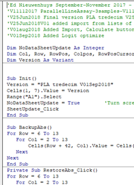
De PLA gebruikt Visual Basic for Application (VBA)
algoritmes. De PLA-berekening en de bijbehorende statistiek wordt
in de Sample 1-13 sheets uitgevoerd. In elke Sample sheet is rechts van de
grafiek de formules te vinden. |
The PLA uses Visual Basic for Application (VBA)
algorithms. The PLA calculation and it statistics is performed in
the Sample 1-13 sheets. The formulas can be found to the right of the graph in
each Sample sheet. |
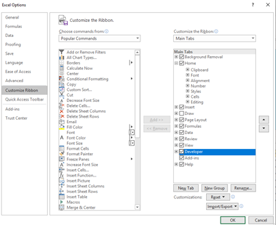
|
Om de VBA algoritmen te zien moet in Excel de optie
Developer in de ribbon aangezet worden. |
To see the VBA coding Developer mode must be turned
on in the ribbon. |
|
|
|
|
|
|
5.2. Praktische uitvoering
|
Open in Excel “PLA
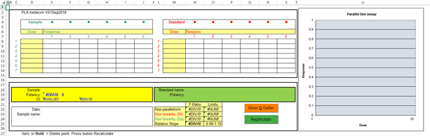
tredecimV01Sep2018.xlsm”. Het volgende scherm wordt getoond. |
Open in Excel "PLA tredecimV01Sep2018.xlsm". The following screen is displayed. |
|
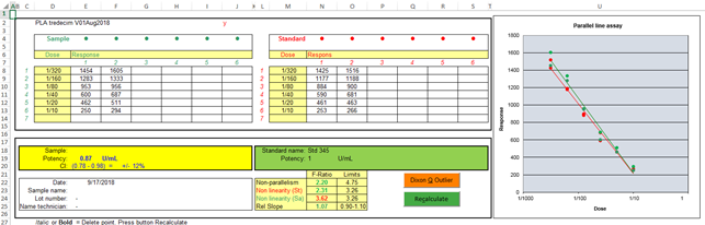
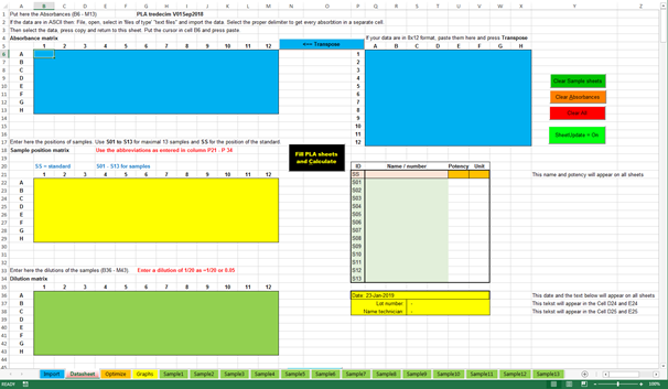
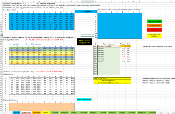
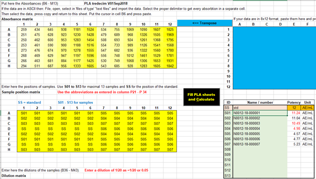
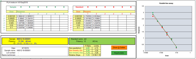
Dit is het invoer- en resultatenscherm. Hierin wordt de inzetdefinitie
vastgelegd en gekoppeld aan de gemeten responses van een ELISA-plaat. Per monster kunnen bij maximaal zeven doses/verdunningen zes responses
worden vastgelegd. Onderin het scherm staan diverse tabbladen. |
This is the input and result screen. Herein, the
deployment definition is recorded and linked to the measured responses of an
ELISA plate. Six responses per sample can be recorded for up to
seven doses / dilutions. At the bottom of the screen there are various tabs. |
x
![]()
|
Het is ook mogelijk om de testen met de hand in te voeren. Druk op Sample1 of een andere groene tab tot en met sample13. Zie hoofdstuk: “Handmatig invoeren” |
It is also possible to
manually enter the tests. Press Sample1 or another green tab up to and
including sample13. |

5.2.1.
Import sheet
|
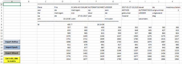
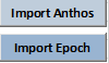
Met dit tabblad kunnen ELISA-reader bestanden ingelezen worden. |
ELISA reader files can be read with this tab. |
|
Er zijn knoppen voor een paar gangbare ELISA-readers gemaakt. Als het
bestand is ingelezen worden de extincties op de juiste plek in de Datasheet
geplaatst. |
|
There are buttons for the some ELISA readers. Once
the file has been read in, the extinctions are placed in the right place in
the Datasheet. |
|
De meetgegevens blijven in het Import tabblad staan zodat het
originele bestand niet verloren gaat. |
The measurement data remains in the Import sheet so
the original file is not lost. |
|
||
|
De “Import wizard” knop is om files van de Wizard
gamma-scintillatieteller in te lezen. |
|
The "Import wizard" button imports files from the
Wizard gamma scintillation counter. |
|||
|
De “List in B1..B96 to matrix”-knop kopieert de alle
waarden uit de range B1..B96 naar de
Absorbance matrix in het Tabblad Datasheet van A1 naar A12, B1 naar
B12, en zo voort. |
|
The “List in B1..B96 to matrix” button copies all
values from the range B1..B96 to the Absorbance matrix in the Datasheet tab
from A1 to A12, B1 to B12, and so on. |
|||
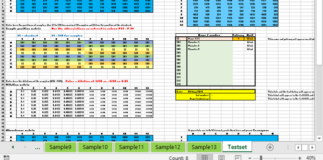
5.2.2.
Datasheet
sheet
|
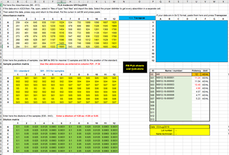
In de “Datasheet” wordt de inzetdefinitie vastgelegd; de positie van
elke verdunning/dosis van elk monster.
Met deze gegevens worden de “sample sheets” met de PLA geladen. Tot 13
“sample sheets” kunnen gevuld worden. |
The deployment definition of an ELISA plate is
recorded in the "Datasheet"; the position of each dilution / dose of each
sample. With this data the "sample sheets" are loaded with the PLA. Up to 13 sample sheets can be filled. |
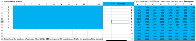
Extincties invoeren
|
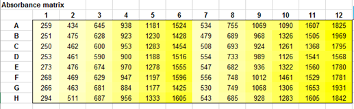
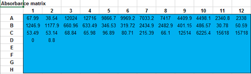
De “Absorbance
matrix” bevat de responses. Bijvoorbeeld extincties of counts. NB. Als de extincties in een 8x12 of 12x8 formaat in een Excel
worksheet zijn opgeslagen dan kunnen de waarden met copy en “paste as values”
in het blauwe vlak gekopieerd worden. |
In the blue "Absorbance matrix" area the responses
are placed. For example extinctions or counts. Calculations are made with the responses in the range
B6: M13. NB. If the absorbances were entered in another Excel
worksheet, the values can be copied with “copy” and “paste as values” in the
blue area. |
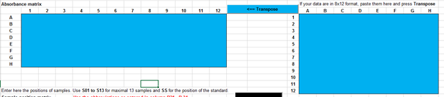

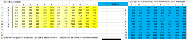
![]()
|
Met de “Transpose” knop kunnen waarden in een 8x12 naar een 12
kolommen bij 8 rijen formaat gekopieerd worden. |
With the “Transpose” button values in a 8x12 format
can be copied to a 12x8 format. |
|
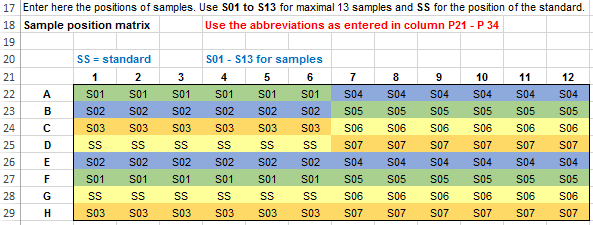
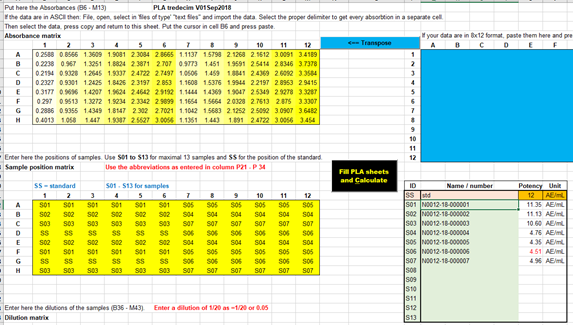
Monstercoderingen invoeren In de “Sample
position” matrix worden de monstercoderingen vastgelegd. De monstercode wordt
in de resultatenoverzicht-tabel aan de werkelijke monsternaam gekoppeld. Gebruik de codering
S01 tot S13 voor de dertien samples. Gebruik SS als codering
voor de standaard. |
Entering Sample
codes Sample codes are recorded in the "Sample position"
matrix. The sample code is linked to the real sample name in
the result overview table. Use the coding S01 to S13 for the
thirteen samples. Use SS as the standard encoding. |
|
|
|
|
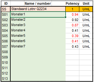
Resultatenoverzichtstabel In het
resultatenoverzichtstabel komt de S01
.. S13-codering weer terug en wordt er een monsternummer of monsternaam
aan gekoppeld. |
Result overview table The S01 .. S13 coding returns in the result overview
table and a sample number or sample name is linked in this table to it. |
|
|
|
|
In deze tabel moet
de naam, lotnummer en concentratie of potency van de gebruikte standaard
achter de ID SS getikt worden. |
In this screen the name, lot number and concentration
or potency of the standard used must be entered after the ID SS. |
|
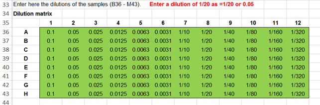
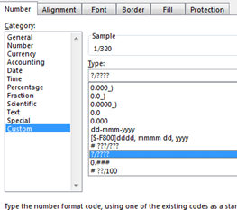
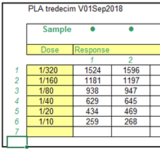
Verdunningen invoeren In de “Dilution
matrix” worden verdunningen vastgelegd. Dat kan in twee formaten; als nummer of als fractie.
De formaten zijn in Excel zelf in te stellen. Houd er rekening mee dat grote verdunningen, zoals 1/5000, 1/10000, de waarde niet goed in de cellen meer past Overweeg dan om de waarden van alle doses in de test een factor 1/1000 groter te maken zodat de waarden weer tussen 1 en 1000 liggen. Vermeld dan bij de tabel “Verdunning * 1000” In de template is
een “custom” formaat van ??/???? ingesteld. In de sample sheets
is de fractie als default formaat geselecteerd. Als dit gewijzigd moet worden selecteer dan Sample1 sheet, houd de
Shift-toets ingedrukt en selecteer Sample13. |
Entering dilutions Dilutions are recorded in the "Dilution matrix". This is possible in two formats; as a number or as a
fraction. The formats can be changed in Excel itself. Keep in mind that large dilutions, such as 1/5000, 1/10000, the value
no longer fits well in the cells. Then consider increasing the values of all doses in the test by
a factor of 1/1000 so that the values are again between 1 and 1000. In the template is a "custom" format of ?? / ???? is
made. |
![]()
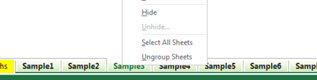
|
Alle dertien tabs worden dan lichter van
kleur. Verander de formats. Klik met rechter muistoets op een tabblad en
kies Ungroup Sheets |
All thirteen tabs will then become lighter in colour.
Change the formats. Right-click on a tab and choose
Ungroup Sheets |
|
waarna alle tabbladen weer groen kleuren. jn. |
after which all tabs turn green again |
![]()
|
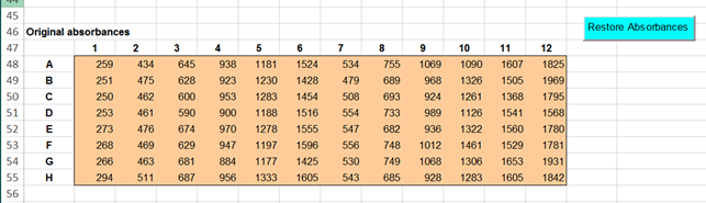
Originele ruwe data terugzetten Onderin de sheet “Datasheet” worden de origineel ingelezen ruwe data
bewaard. Door op de knop “Restore Absorbances” te drukken worden deze naar de
“Absorbance matrix” boven in de sheet gekopieerd. |
Restore original data At the bottom of the "Datasheet" sheet, the
originally imported raw data are saved. By pressing the "Restore Absorbances" button, these
are copied to the "Absorbance matrix" at the top of the sheet. |
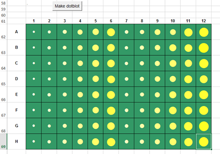
|
Dotblot De ingelezen extincties worden in de “Absorbance matrix” naar gelang
hun sterkte donkerder gekleurd. Met de dotblot wordt de sterkte met een
cirkelgroote en kleur-intensiteit weergegeven |
Dot blot The absorbed readings are coloured in the "Absorbance
matrix" according to their strength. With the dot blot the strength is shown
with a circle size and colour intensity. |
5.2.3.
Optimize sheet
|
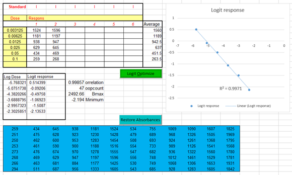
Voor een PLA moeten beide
dose-respons lijnen recht zijn. Vaak moet het meetgebied verkort worden omdat anders de F-ratio voor lineariteit buiten de
specificaties valt. Door de vaak sigmoïde lijn recht te maken kan een logit-transformatie
op de responses van de standaard de kromme lijnen recht maken. De gemiddelde responses van de standaard van Sample1 worden met een
logit-functie log(y / 1 - y) gelineariseerd. Met de berekende formule log(response / (Bmax-response)) worden daarna
alle responses geconverteerd. Daarna wordt van alle responses met de laagste waarde van de
logit-regressie (Minimum) afgetrokken zodat geen negatieve getallen ontstaan.
Dit voorkomt vreemde grafieken en verkeerde beslissingen in de software die
test op positieve getallen. In het voorbeeld hieronder zijn 3 samples afgekeurd op lineariteit. |
For a PLA, both dose-response lines must be straight.
Often the measuring range has to be shortened because
otherwise the F-ratio for linearity falls outside the specifications. By straightening the often sigmoid line, a logit
transformation on the responses of the standard can straighten the curved
lines. The average responses of the Sample1 standard are
linearized with a logit function log (y / 1 - y). With the calculated formula log (response /
(Bmax-response)), all responses are then converted. Subsequently, all responses with the lowest value of
the logit regression (Minimum) are subtracted so that no negative numbers
arise. This prevents strange graphs and wrong decisions in the software that
tests for positive numbers. In the example below three samples are rejected on
linearity |
|
Deze functie transformeert de dose-responses van de standaard met een
logit-transformatie naar een rechte lijn met de formule: Logboek (antwoord / (Rmax - antwoord)). Het algoritme zoekt een Rmax dat de hoogste correlatie oplevert. Hoe hoger de correlatie hoe rechter de lijn zal zijn. Na optimalisatie worden de getransformeerde gegevens gekopieerd naar
de absorbtiematrixtabel in het gegevensblad. Druk de knop “Fill PLA sheets and Calculate” om de PLA te berekenen. De originele meetgegevens kunnen weer teruggezet worden met de knop
“Restore Absorbances”. |
This function transforms the dose-responses of the
standard with a logit transformation to a linear line with the formula: Log (response / (Rmax - response)). The algorithm searches for an Rmax that gives the
highest correlation. The higher the correlation the more linear the line will
be. After optimisation the transformed data are copied to
the Absorbance matrix table in the Datasheet sheet. Press the button “Fill PLA sheets and Calculate” to
perform the PLA calculations The original data can be restored by pressing the
button “Restore Absorbances”. |
|
Optimaliseert de
response van de standaard van Sample1 tot een rechte lijn. Zet de oorspronkelijke responses weer terug en wist de berekende
potencies in de Datasheet. Druk in na een “Logit Optimize” of na herstel van de originele
responses weer op de knop om de PLA uit te voeren over alle monsters. |
|
Optimizes the response of the standard of Sample1 to
a straight line. Put the original responses back and erase the
calculated potencies in the Datasheet. After a “Logit Optimize” or after restoring the
original responses, press this button again to execute the PLA on all samples. |
5.2.4.
Graphs sheet
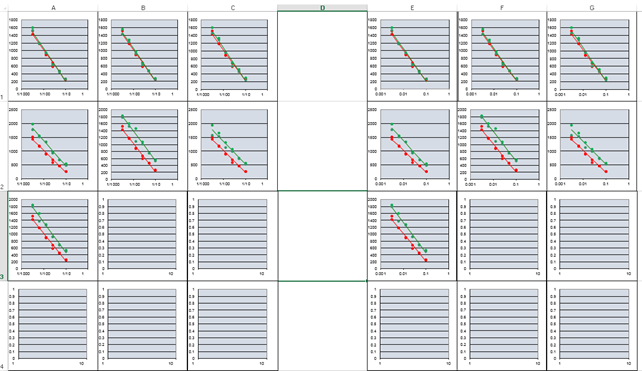
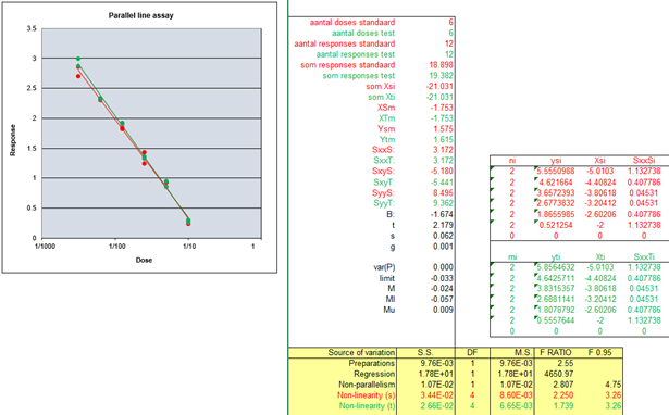
|
In dit tabblad is een overzicht van de PLA-grafieken van alle dertien
monsters. In de linker helft van de verdunningen als fractie (1/20, 1/100) en in
de rechter helft als decimaal getal (0.05, 0.01). De grafieken die niet gebruikt worden kunnen gewist worden zonder dat
het berekeningen beïnvloed. |
This sheet is
an overview of all PLA-graphs of the thirteen samples. In the left half the dilutions as a fraction (1/20,
1/100) and in the right half the same graph as a decimal number (0.05, 0.01). The graphs that are not used can be deleted without
affecting calculations. |
5.2.5.
Sample sheets
|
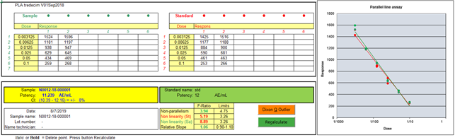
De gegevens van elk van de dertien monsters wordt in een eigen tabblad
gekopieerd. Elk tabblad heeft zijn eigen formules voor de berekening van de
PLA. De tabbladen zijn daardoor afzonderlijk te gebruiken en beïnvloeden
elkaar niet. Dit betekent dat als bij de standaard een punt ongelding wordt gemaakt
dit niet bij de overige monsters gebeurd. Meetpunten kunnen ongeldig worden gemaakt door de respons bold of italic te maken. Als daarna |
Each of the thirteen samples has its own sheet with
calculations, graph and results. Therefor calculations of the samples can be treated
individual. Removal of a measurement of the standard only
influences the results of that particular sample and not the result of the
remaining twelve samples. Measuring points can be made invalid if the response
is made bold or italic. After pressing |
![]()
|
Als een punt weer valide moet worden gemaakt kan het bold of italic
weer ongedaan worden gemaakt en zal na een “Recalculate” de streep door de
respons weer verdwijnen. Het meetpunt wordt weer in de grafiek getoond worden en in de
PLA-berekening worden op nieuw uitgevoerd. |
If a measuring point has to be made valid again, the
bold of italic font can be undone again. After a “Recalculate” the strikethrough line will disappear. The measuring point will be shown again in the graph
and used in the PLA calculation. |
![]()
|
Met de Dixon Q Outlier-test kunnen uitbijters gedetecteerd en
verwijderd worden. |
The Dixon Q outlier test can be used to remove
outliers. |
'From
wikipedia
'In
statistics, Dixon's Q test, or simply the Q test, is used for identification and
rejection of outliers.
'This
assumes normal distribution this
test should be used sparingly and never more than once in a data set.
'To
apply a Q test for bad data, arrange the data in order of increasing values and
calculate Q as defined:
'Q =
Gap / Range
'Where
Gap Is the difference between the outlier in question and the closest number to
it.
'If Q
> Qtable, where Qtable is a reference value corresponding to the sample size and
confidence level,
'then
reject the questionable point. Note that only one point may be rejected from a
data set using a Q test.
'Example
'Consider the data set:
'0.189
, 0.167 , 0.187 ,
0.183 , 0.186 , 0.182 ,
0.181 , 0.184 , 0.181 ,
0.177
'Now
rearrange in increasing order:
'0.167
, 0.177 , 0.181 ,
0.181 , 0.182 , 0.183 ,
0.184 , 0.186 , 0.187 ,
0.189
'We
hypothesize that 0.167 is an outlier. Calculate Q:
'Q = gap range = 0.177 - 0.167 / 0.189 - 0.167 = 0.455.
'With
10 observations and at 90% confidence, Q = 0.455 > 0.412 = Qtable, so we
conclude 0.167 is an outlier.
'However, at 95% confidence, Q = 0.455 < 0.466 = Qtable 0.167 is not considered
an outlier.
'This
means that for this example we can be 90% sure that 0.167 is an outlier, but we
cannot be 95% sure.
'This
table summarizes the limit values of the test.
'
Number of values:
' 3
4 5 6
7 8 9
10
'Q90: 0.941, 0.765, 0.642, 0.560, 0.507, 0.468,
0.437, 0.412,
'Q95: 0.970, 0.829, 0.710, 0.625, 0.568, 0.526,
0.493, 0.466,
'Q99: 0.994, 0.926, 0.821, 0.740, 0.680, 0.634,
0.598, 0.568
5.2.6.
Testset sheet
|
Op dit tabblad staan twee testsets. Voordat de testdata naar de Datasheet gekopieerd kunnen worden moet de
knop “Datasheetupdate” in de Datasheet van = On naar = Off gezet worden. |
This sheet contains data of two test sets. Before the test data can be copied to the Datasheet,
the button "Datasheet update" in the Datasheet must be switched from
= On to = Off. |
![]()
![]()
|
De PLA Excel workbook controleert voortdurend of gegevens veranderen.
Dit blokkeert kopiëren en plakken tussen de sheets. De knop “SheetUpdate” zet dit controleren uit of aan. Een andere optie is om de testset eerst naar een lege Excel te
kopiëren en daarna met copy en paste naar de PLA datasheet. |
The PLA Excel workbook constantly checks whether data
changes. The "SheetUpdate" button turns this check on or off. Another option is to first copy the test set to an
empty Excel and then with copy and paste to the PLA datasheet. |
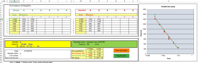
5.2.7.
Handmatig invoeren / Manual entry
|
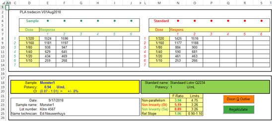
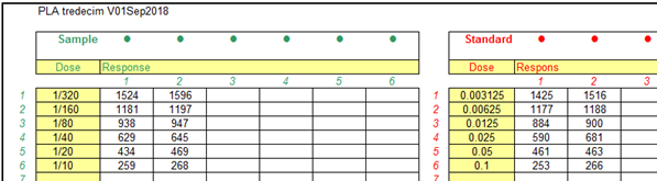
Druk op een groene tab onderin het scherm. Er kunnen dertien van deze identieke tabbladen geopend worden. Elk tabblad heeft zijn eigen PLA-berekeningen die te zien zijn rechts
van de grafiek. Alleen de berekeningen achter de knoppen “Dixon Q Outlier” en
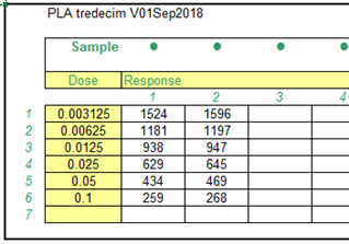
Recalculate zijn in Visual basic (VBA) geschreven. Het volgende scherm wordt zichtbaar |
Press one of the green tabs at the bottom of the
screen. Thirteen of these identical sample tabs can be
opened. Each tab has its own PLA calculations that can be
seen to the right of the graph. Only the calculations behind the “Dixon Q Outlier”
and Recalculate buttons are written in Visual basic (VBA).The following screen
appears |
|
Vul in de kolom onder “Dose” de verdunning (1/16) in of hoeveelheid toegevoegd materiaal, bijvoorbeeld ul’s. |
Enter the dilution (1/16) or amount of added
material, for example ul’s in the column "Dose". |
|
Verdunning kunnen ook als fractie (1/16) zichtbaar gemaakt worden. Bij “format cell -> custom” is een extra formaat ?/???? toegevoegd die
verdunning tot 1/9999 kan laten zien. Hier kan ook nog bijvoorbeeld ??/?????? toevoegen zodat een verdunning
van bijvoorbeeld 22/123456 getoond kan worden |
It is possible to make the dilution visible as a
fraction (1/16). With "format cell -> custom" is an additional format?
/ ???? added which displays dilutions up to 1/9999. Also possible, for example is ?? / ?????? so that a
dilution of, for example, 22/123456 can be shown |
|
Vul de gemeten waarden, responses ,achter de juiste dosis, in het blok
“Response”. |
Enter the measured values, responses, behind the
proper dosis, in the "Response" |
|
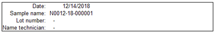
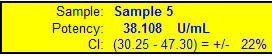
De naam en de potency of activiteit van de standaard wordt in deze
velden ingevoerd. |
The name and potency or activity of the standard are
entered in these fields. |
![]()
|
De naam van het monster, testdatum et cetera kunnen
in deze velden worden ingevoerd. |
The sample name, test date, etc. can be entered in
these fields. |
|
Responses kunnen ongeldig worden gemaakt door de respons bold
of italic te maken. Als daarna |
Responses can be invalidated by making the response
bold
or italic. If |
![]()
|
Als een punt weer valide moet worden gemaakt kan het bold of italic
weer ongedaan worden gemaakt en zal na een “Recalculate” de streep door de
respons weer verdwijnen. Het meetpunt wordt weer in de grafiek getoond worden en in de
PLA-berekening worden op nieuw uitgevoerd. |
If a measuring point has to be made valid again, the
bold of italic font can be undone again. After a “Recalculate” the strikethrough line will
disappear. The measuring point will be shown again in the graph
and used in the PLA calculation. |
![]()
|
Met de Dixon Q Outlier-test kunnen uitbijters gedetecteerd en
verwijderd worden. |
The Dixon Q outlier test can be used to remove
outliers. |
'From wikipedia
'In statistics, Dixon's Q test, or simply the Q
test, is used for identification and rejection of outliers.
'This assumes normal distribution this test should be used sparingly and
never more than once in a data set.
'To apply a Q test for bad data, arrange the
data in order of increasing values and calculate Q as defined:
'Q = Gap / Range
'Where Gap Is the difference between the outlier
in question and the closest number to it.
'If Q > Qtable, where Qtable is a reference
value corresponding to the sample size and confidence level,
'then reject the questionable point. Note that
only one point may be rejected from a data set using a Q test.
'Example
'Consider the data set:
'0.189 ,
0.167 , 0.187 , 0.183 ,
0.186 , 0.182 , 0.181 ,
0.184 , 0.181 , 0.177
'Now rearrange in increasing order:
'0.167 ,
0.177 , 0.181 , 0.181 ,
0.182 , 0.183 , 0.184 ,
0.186 , 0.187 , 0.189
'We hypothesize that 0.167 is an outlier. Calculate Q:
'Q = gap range
= 0.177 - 0.167 / 0.189 - 0.167
= 0.455.
'With 10 observations and at 90% confidence, Q =
0.455 > 0.412 = Qtable, so we conclude 0.167 is an outlier.
'However, at 95% confidence, Q = 0.455 < 0.466 =
Qtable 0.167 is not considered an outlier.
'This means that for this example we can be 90%
sure that 0.167 is an outlier, but we cannot be 95% sure.
'This table summarizes the limit values of the
test.
' Number of values:
'
3
4 5
6 7 8
9 10
'Q90: 0.941, 0.765, 0.642, 0.560, 0.507, 0.468, 0.437, 0.412,
'Q95: 0.970, 0.829, 0.710, 0.625, 0.568, 0.526, 0.493, 0.466,
'Q99: 0.994, 0.926, 0.821, 0.740, 0.680, 0.634, 0.598, 0.568
5.3. Beoordeling resultaten
|
Als punten ongeldig moeten worden gemaakt kan
dat door ze te verwijderen. Dit heeft als groot nadeel dat niet meer te zien
is wat de respons was van het verwijderde meetpunt. Een betere methode is om het te verwijderen
punt bold of italic te maken en daarna op de groene knop “Recalculate” te drukken. De respons verdwijnt wel uit de grafiek maar
is nog wel zichtbaar in de invoertabel. Weghalen van uitbijters ‘op het oog’ is
discutabel.
Of helemaal geen punten weghalen en de test
te herhalen. Realiseer je dat de statistiek ‘unbalanced’
wordt als meetpunt verwijderd worden. De variantieanalyse gaat er van uit dat
alle punten aanwezig zijn. De parallelliteit en de lineariteit van de
twee lijnen en worden beoordeeld door F-toetsen die berekend woorden door
middel van variantieanalyse (ANOVA). Zie
hoofdstuk 2.2 Principe |
If measuring points have to
be invalided, it is possible to erase it. This has the disadvantage it
is impossible to see what the response was if the deleted measuring point. A better method is to make
the response bold or italic and press the green “Recalculate”
button. The response disappears from
the graph but is still visible in the input table. Invalidating outliers ‘by
eye’ is debatable. It is better to use the Dixon
Q outlier test. Or preferable; don't remove
points at all and repeat the test. Realise that the statistic
becomes "unbalanced" when measurement points are deleted. The variance
analysis assumes that all points are present. Parallelism and linearity of the
two lines are tested by F-tests calculated by means of analysis of variance (ANOVA). See chapter 2.2 Principle |
|
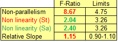
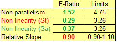
Er kunnen een of meerdere criteria gehanteerd worden om de resultaten
te beoordelen. F-toetsen: Als een F-ratio groter is dan de Limit, ook wel F-norm, genoemd dan
geeft dat aan de de helling van de standaard en monster niet overeenkomen of
dat de lijn van de standaard rechter is dan die van het monster. St slaat op de
standaard en Sa op het monster (Sample). |
One or more criteria can be used to assess the
results. F-tests: If an F-ratio is exceeds the Limit, also called the
F-norm, it indicates that the regression line have different slopes or the
standard is more linear than the sample regression line. St refers to the standard and
Sa
to the sample. |
|
Relatieve slope: Als de hellingen van standaard en monster (relative slope) meer dan 10% van elkaar
afwijken duidt dat op een probleem in de test. In bijna alle gevallen is de F-test op non-parallelism dan ook
afwijkend. |
Relative slope: If the slopes of the standard and sample (relative
slope) deviates more than 10% from
each other it is due to a a problem in the test. In almost all cases the F test on non-parallelism is
also out of specification. |
.
|
De betrouwbaarheid van het
resultaat: Als de reproduceerbaarheid van de meetpunten per dosis slecht is
kunnen alle F-toetsen binnen de norm blijven maar is het resultaat
onbetrouwbaar. Dit komt tot uitdrukking in de CI (confidence interval) dat ook
als percentage ten opzichte van het gemiddelde berekend wordt. Afhankelijk van de gewenste betrouwbaarheid van het resultaat kan hier
een grens voor worden gesteld. Grenzen tussen de 10% en 20% zijn gangbaar. |
The reliability of the result: If the reproducibility is poor of the measurement
points per dose, all F-tests can remain below the norm, but the result will be
unreliable. This is expressed in the CI (confidence interval) of
the potency (result). The confidence interval is also calculated as a
percentage relative to the potency. Depending on the desired reliability, a limit can be
set for the CI. Limits between 10% and 20% are common. |
6.
Literature
|
David J. Finney |
Statistical Method in biological assay, Third edition 1978, Pag 69-132 |
7.
Attachments

PLA
tredecim als Excel-applicatie: 27-Dec-2018
01:09:18
Dubbelklik op te openen / double click to open